Logistic回归

gavinhome

2017-08-26

机器学习

Logistic回归回归又称Logistic回归回归分析，是一种广义的线性回归分析模型，常用于数据挖掘，疾病自动诊断，经济预测等领域。

分类问题的首选算法。
Logistic回归解决二分类问题，Softmax回归解决多分类问题。

Sigmoid函数

$$g\left(z\right) = \frac{1}{1+e^{-z}}=h_\theta \left(x\right) =g\left ( \theta ^Tx \right )=\frac{1}{1+e^{-\theta ^T x}}$$

$${g}’\left ( x \right ) = {\left ( \frac{1}{1+e^{-x}} \right )}’=\frac{e^{-x}}{\left ( 1+e^{-x} \right )^2}=\frac{1}{1+e^{-x}}\cdot \left ( 1- \frac{1}{1+e^{-x}} \right )=g\left ( x \right )\cdot \left ( 1-g\left ( x \right ) \right )$$

Logistic回归参数估计

假定：
$$P\left ( y=1|x;\theta \right ) = h_\theta \left ( x \right )$$,
$$P\left ( y=0|x;\theta \right ) = 1-h_\theta \left (x \right)$$

则：
$$P\left(y|x;\theta\right)=\left(h_\theta\left(x\right )\right)^y\left(1-h_\theta\left(x\right)\right)^{1-y}$$

似然函数：
$$L\left ( \theta \right ) = p\left ( \vec{y}|X;\theta \right ) = \prod_{i = 1}^{m}p\left ( y^\left ( i \right ) \right | {x^\left ( i \right )};\theta ) = \prod_{i=1}^{m}{\left ( h_\theta \left ( x^{\left ( i \right )} \right ) \right )^{y^\left ( i \right ) }} {\left ( 1-h_\theta\left ( x^\left ( i \right ) \right ) \right )^{1-y^\left ( i \right )}}$$

取对数得到：$$l\left ( \theta \right ) = logL\left ( \theta \right ) = \sum_{i=1}^{m}y^{\left ( i \right )}logh\left ( x^\left ( i \right ) \right ) + \left ( 1-y^\left ( i \right ) \right ) log\left ( 1-h\left ( x^\left ( i \right ) \right ) \right )$$

最后，对$$\theta$$参数求偏导：

$$\frac{\partial l\left ( \theta \right )}{\partial \theta_j} = \sum_{i=1}^{m}\left ( y^{\left ( i \right ) } -g\left ( \theta^Tx^{\left ( i \right )} \right )\right )\cdot x_j^{\left ( i \right )}$$

参数迭代

Logistic回归参数的学习规则：

$$\theta_j: = \theta_j + \alpha \left ( y^{\left ( i \right )} - h_\theta\left ( x^{\left ( i \right )} \right )\right )x_j^{\left ( i \right )}$$

损失函数

$$\therefore loss\left ( y_i,\hat{y}_i \right ) = -l\left ( \theta \right )$$，其中$$y_i\in \left { 0,1 \right }$$,$$\hat{y} = \left{\begin{matrix}
p_i & y_i=1 \
1-p_i & y_i = 0
\end{matrix}\right.$$

带入推导可得最终损失函数：$$\therefore loss\left ( y_i,\hat{y}i \right ) = -l\left ( \theta \right ) = - \sum{i=1}^{m}ln\left [ p_i^{y_i}\left ( 1-p_i \right )^{1-y_i} \right ] = \sum_{i=1}^{m}ln\left [ y_iln\left ( 1+e^{-f_i} \right ) + \left ( 1-y_i \right )ln\left ( 1+e^{f_i} \right )\right ]$$

Logistic回归的损失

$$y_i\in \left { -1,1 \right }$$

$$L\left ( \theta \right ) = \prod_{i=1}^{m}P_i^{\frac{\left ( y_i + 1 \right)}{2}}\left ( 1-P_i\right )^{\frac{-\left ( y_i-1 \right )}{2}}$$

$$loss\left ( y_i,\hat{y_i} \right )=\sum_{i=1}^{m}\left [ ln\left ( 1+e^{-y_i\cdot f_i} \right ) \right ]$$

广义线性模型Generalized Linear Model

y不再只是正太分布，而是扩大为指数族中的任一分布；
x -> g(x) -> y,连接函数g单调可导，例如逻辑回归中的$$g\left ( z \right ) = \frac{1}{1+e^{-z}}$$，拉伸变换$$g\left(z\right )=\frac{1}{1+e^{-\lambda z}}$$

GLM

Softmax回归

K分类，第k类的参数为$$\vec{\theta_k}$$，组成二维矩阵$$\theta _{k\times n}$$
概率：$$p\left ( c=kx;\theta\right)=\frac{exp\left ( \theta_k^T x \right )}{\sum_{l=1}^{K}exp\left ( \theta_l^T x \right )}$$, 其中k=1,2,……,K
似然函数：$$ L\left ( \theta \right ) =\prod_{l=1}^{m}\prod_{k=1}^{K} p\left (c=k|x^{\left ( i \right )} ;\theta \right )^{y_k^\left ( i \right )}
=\prod_{l=1}^{K}\prod_{k=1}^{K}\left( exp\left ( \theta_k^T x^{\left ( l \right )} \right ) / \sum_{l=1}^{K}exp\left ( \theta^T_l x^\left ( l \right ) \right )\right )^{y_k^{\left ( i \right )}} $$
对数似然：
$$J_m\left ( \theta \right ) = ln L\left ( \theta \right ) = \sum_{i=1}^{m}\sum_{k=1}^{K}y_k^{\left ( i \right )}\cdot \left ( \theta^T_kx^{\left ( i \right )} - ln \sum_{l=1}^{K}exp\left ( \theta^T_l x^{\left ( i \right )} \right )\right )$$，
$$J\left ( \theta \right ) = \sum_{k=1}^{K}y_k\cdot \left ( \theta^T_k x - ln\sum_{l=1}^{K}exp\left ( \theta_l^Tx \right )\right )$$
随机梯度：
$$\frac{\partial J\left ( \theta \right )}{\partial \theta_k} = \left ( y_k - p\left ( y_k|x,\theta \right ) \right )\cdot x$$

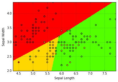
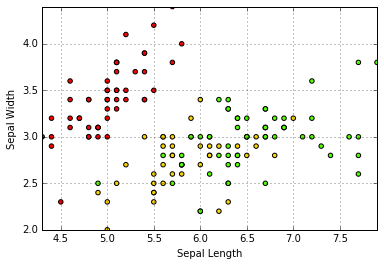
鸢尾花分类

实验数据

鸢尾花数据集是最有名的模式识别测试数据，1936年模式识别先驱Fisher在其论文“The use of multiple measurements in taxonomic problems” 使用了它。数据集包括3个鸢尾花类别，每个类别有50个样本，其中一个类别与另外两类线性可分，而另外两类不能线性可分。

数据描述

该数据集包括150行，每行为1个样本，每个样本共有5个字段，分别是花萼长度，花萼宽度，花瓣长度，花瓣宽度，类别。其中类别包括Iris Setosa, Iris Versicolour,Iris Virginica三类，前四个字段的单位为cm。

实验代码

# -*- coding: utf-8 -*
import pandas as pd
import io
import requests
import matplotlib as mpl # 设置环境变量
import matplotlib.pyplot as plt # 绘图专用
from sklearn.cross_validation import train_test_split
from sklearn import metrics
import numpy as np
from sklearn.linear_model import LogisticRegression
import sys
reload(sys)
sys.setdefaultencoding('utf8')
mpl.rcParams['font.sans-serif'] = ['FangSong']
mpl.rcParams['axes.unicode_minus']=False

def iris_type(s):
    it = {'Iris-setosa':0,'Iris-versicolor':1,'Iris-virginica':2}
    return it[s]

url="http://archive.ics.uci.edu/ml/machine-learning-databases/iris/iris.data"
data = pd.read_table(io.StringIO(requests.get(url).content.decode('utf-8')), sep=" ", delimiter=',', dtype=float, converters={4:iris_type}, header=None,names=['a','b','c','d','e']).values
# print data
# print type(data)

x,y = np.split(data,(4,),axis=1)
x=x[:,:2]
#print x

logreg = LogisticRegression()
logreg.fit(x,y.ravel())

N, M = 500, 500
x1_min, x1_max = x[:,0].min(),x[:,0].max()
x2_min, x2_max = x[:,1].min(),x[:,1].max()
t1 = np.linspace(x1_min,x1_max,N)
t2 = np.linspace(x2_min,x2_max,M)

x1,x2 = np.meshgrid(t1, t2)
x_test = np.stack((x1.flat,x2.flat), axis=1)

y_hat = logreg.predict(x_test)
y_hat = y_hat.reshape(x1.shape)
plt.pcolormesh(x1,x2,y_hat,cmap=plt.cm.prism)
plt.scatter(x[:,0],x[:,1], c=y, edgecolors='k',cmap=plt.cm.prism)
plt.xlabel('Sepal Length')
plt.ylabel('Sepal Width')
plt.xlim(x1_min, x1_max)
plt.ylim(x2_min, x2_max)
plt.grid()
plt.show()

png


y_hat = logreg.predict(x)
y = y.reshape(-1)

print y_hat.shape
print y.shape
result = y_hat == y
print y_hat
print y
print result
c=np.count_nonzero(result)
print c
'Accuracy: %.2f%%' % (100*float(c)/float(len(result)))

'Accuracy: 76.67%'

结果分析

仅用花萼长度和宽度，在150个样本中，有115个分类正确，正确率为76.67%
使用四个特征，试验后发现有144个样本分类正确，正确率为96%.

案例跟踪

# -*- coding: utf-8 -*
import pandas as pd
import io
import requests
import matplotlib as mpl # 设置环境变量
import matplotlib.pyplot as plt # 绘图专用
from sklearn.model_selection  import train_test_split
from sklearn.linear_model import LinearRegression
from sklearn import metrics
import numpy as np
from sklearn.linear_model import LogisticRegression
import sys
reload(sys)
sys.setdefaultencoding('utf8')
mpl.rcParams['font.sans-serif'] = ['FangSong']
mpl.rcParams['axes.unicode_minus']=False

def iris_type(s):
    it = {'Iris-setosa':0,'Iris-versicolor':1,'Iris-virginica':2}
    return it[s]

url="http://archive.ics.uci.edu/ml/machine-learning-databases/iris/iris.data"
data = pd.read_table(io.StringIO(requests.get(url).content.decode('utf-8')), sep=" ", delimiter=',', dtype=float, converters={4:iris_type}, header=None,names=['a','b','c','d','e']).values
# print data
# print type(data)

x,y = np.split(data,(4,),axis=1)
X=x[:,:4]

x1_min, x1_max = x[:,0].min(),x[:,0].max()
x2_min, x2_max = x[:,1].min(),x[:,1].max()

plt.scatter(x[:,0],x[:,1], c=y, edgecolors='k',cmap=plt.cm.prism)
plt.xlabel('Sepal Length')
plt.ylabel('Sepal Width')
plt.xlim(x1_min, x1_max)
plt.ylim(x2_min, x2_max)
plt.grid()
plt.show()

X_train,X_test,y_train,y_test = train_test_split(X,y,random_state=1)
linreg = LogisticRegression()
model = linreg.fit(X_train,y_train)
y_pred = linreg.predict(X_test)
# print linreg.coef_

result = y_pred == y_test.ravel()

c=np.count_nonzero(result)